First Derivative of the Multivariate Normal Densities with RcppArmadillo

Joscha Legewie — written Sep 9, 2013 — source

There is a great RcppArmadillo implementation of multivariate normal densities. But I was looking for the first derivative of the multivariate normal densities. Good implementations are surprisingly hard to come by. I wasn’t able to find any online and my first R implementations were pretty slow. RcppArmadillo might be a great alternative particularly because I am not aware of any c or Fortran implementations in R. In these areas, we can expect the largest performance gains. Indeed, the RcppArmadillo version is over 400-times faster than the R implementation!

First, let’s take a look at the density function \(x \sim N(m,\Sigma)\) as shown in the The Matrix Cookbook (Nov 15, 2012 version) formula 346 and 347

\[\frac{\partial p(\mathbf{x})}{\partial\mathbf{x}}=-\frac{1}{\sqrt{det(2\pi\mathbf{\Sigma})}}exp\left[-\frac{1}{2}(\mathbf{x}-\mathbf{m})^{T}\mathbf{\Sigma}^{-1}(\mathbf{x}-\mathbf{m})\right]\mathbf{\Sigma}^{-1}(\mathbf{x}-\mathbf{m})\]

where \(\mathbf{x}\) and \(\mathbf{m}\) are d-dimensional and \(\mathbf{\Sigma}\) is a \(d \times d\) variance-covariance matrix.

Now we can start with a R implementation of the first derivative of the multivariate normal distribution. First, let’s load some R packages:

library('RcppArmadillo')
library('mvtnorm')
library('rbenchmark')
library('fields')

Here are two implementations. One is pure R and one is based on dmvnorm in the mvtnorm package.

dmvnorm_deriv1 <- function(X, mu=rep(0,ncol(X)), sigma=diag(ncol(X))) {
    fn <- function(x) -1 * c((1/sqrt(det(2*pi*sigma))) * exp(-0.5*t(x-mu)%*%solve(sigma)%*%(x-mu))) * solve(sigma,(x-mu))
    out <- t(apply(X,1,fn))
    return(out)
}
dmvnorm_deriv2 <- function(X, mean, sigma) {
    if (is.vector(X)) X <- matrix(X, ncol = length(X))
    if (missing(mean)) mean <- rep(0, length = ncol(X))
    if (missing(sigma)) sigma <- diag(ncol(X))
    n <- nrow(X)
    mvnorm <- dmvnorm(X, mean = mean, sigma = sigma)
    deriv <- array(NA,c(n,ncol(X)))
    for (i in 1:n)
        deriv[i,] <- -mvnorm[i] * solve(sigma,(X[i,]-mean))
    return(deriv)
}

These implementations work but they are not very fast. So let’s look at a RcppArmadillo version. The Mahalanobis function and the first part of dmvnorm_deriv_arma are based on this gallery example, which implements a fast multivariate normal density with RcppArmadillo.

#include <RcppArmadillo.h>

// [[Rcpp::depends(RcppArmadillo)]]
// [[Rcpp::export]]
arma::vec Mahalanobis(arma::mat x, arma::rowvec center, arma::mat cov){
    int n = x.n_rows;
    arma::mat x_cen;
    x_cen.copy_size(x);
    for (int i=0; i < n; i++) {
        x_cen.row(i) = x.row(i) - center;
    }
    return sum((x_cen * cov.i()) % x_cen, 1);
}

// [[Rcpp::export]]
arma::mat dmvnorm_deriv_arma(arma::mat x, arma::rowvec mean, arma::mat sigma) {
    // get result for mv normal
    arma::vec distval = Mahalanobis(x,  mean, sigma);
    double logdet = sum(arma::log(arma::eig_sym(sigma)));
    double log2pi = std::log(2.0 * M_PI);
    arma::vec mvnorm = exp(-( (x.n_cols * log2pi + logdet + distval)/2));

    // get derivative of multivariate normal
    int n = x.n_rows;
    arma::mat deriv;
    deriv.copy_size(x);
    for (int i=0; i < n; i++) {
        deriv.row(i) = -1 * mvnorm(i) * trans(solve(sigma, trans(x.row(i) - mean)));
    }
    return(deriv);
}

Now we can compare the different implementations using simulated data.

set.seed(123456789)
s <- rWishart(1, 2, diag(2))[,,1]
m <- rnorm(2)
X <- rmvnorm(10000, m, s)

benchmark(dmvnorm_deriv_arma(X,m,s),
          dmvnorm_deriv1(X,mu=m,sigma=s),
          dmvnorm_deriv2(X,mean=m,sigma=s),
          order="relative", replications=10)[,1:4]

                                    test replications elapsed relative
1            dmvnorm_deriv_arma(X, m, s)           10   0.258    1.000
3 dmvnorm_deriv2(X, mean = m, sigma = s)           10   0.962    3.729
2   dmvnorm_deriv1(X, mu = m, sigma = s)           10   4.550   17.636

The RcppArmadillo implementation is several hundred times faster! Such stunning performance increases are possible when existing implementation rely on pure R (or, as in dmvnorm_deriv2, do some of the heavy lifting in R). Of course, the R implementation can probably be improved.

Finally, let’s plot the x- and y- derivates of the 2-dimensional normal density function.

n <- 100
x <- seq(-3,3, length.out = n)
y <- seq(-3,3, length.out = n)
z1 <- outer (x, y , function(x1,x2) dmvnorm_deriv_arma(cbind(x1,x2),rep(0,2),diag(2))[,1])
z2 <- outer (x, y , function(x1,x2) dmvnorm_deriv_arma(cbind(x1,x2),rep(0,2),diag(2))[,2])

par(mfrow=c(1,2),mar=c(0,0,0,0), cex=0.8, cex.lab=0.8, cex.main=0.8, mgp=c(1.2,0.15,0), cex.axis=0.7, tck=-0.01)
drape.plot(x,y,z1,border=NA, add.legend=FALSE, phi=30, theta= 50)
drape.plot(x,y,z2,border=NA, add.legend=FALSE, phi=30, theta= 50)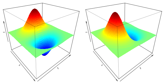

plot of chunk unnamed-chunk-5

Note: This is an updated version dated 2015-01-06 of the original article.

tags: armadillo

Extending R with C++ and Fortran — Dirk Eddelbuettel and JBrandon Duck-Mayr
Benchmarking Rcpp code with RcppClock — Zach DeBruine
Simulation Smoother using RcppArmadillo — Tomasz Woźniak

First Derivative of the Multivariate Normal Densities with RcppArmadillo

Related Articles