Stochastic SIR Epidemiological Compartment Model

Christian Gunning — written Apr 25, 2015 — source

Introduction

This post is a simple introduction to Rcpp for disease ecologists, epidemiologists, or dynamical systems modelers - the sorts of folks who will benefit from a simple but fully-working example. My intent is to provide a complete, self-contained introduction to modeling with Rcpp. My hope is that this model can be easily modified to run any dynamical simulation that has dependence on the previous time step (and can therefore not be vectorized).

This post uses a classic Susceptible-Infected-Recovered (SIR) epidemiological compartment model. Compartment models are simple, commonly-used dynamical systems models. Here I demonstrate the tau-leap method, where a discrete number of individuals move probabilistically between compartments at fixed intervals in time. In this model, the wait-times within class are exponentially distributed, and the number of transitions between states in a fixed time step are Poisson distributed.

This model is parameterized for the spread of measles in a closed population, where the birth rate (nu) = death rate (mu). The transmission rate (beta) describes how frequently susceptible (S) and infected (I) individuals come into contact, and the recovery rate (gamma) describes the the average time an individual spends infected before recovering.

C++ Code

Note: C++ Functions must be marked with the following comment for use in R: // [[Rcpp::export]].

When functions are exported in this way via sourceCpp(), RNG setup is automatically handled to use R’s engine. For details on random number generation with Rcpp, see the this Rcpp Gallery post.

#include <Rcpp.h>
using namespace Rcpp;

// This function will be used in R! Evaluates the number of events
// and updates the states at each time step
//
// [[Rcpp::export]]
List tauleapCpp(List params) {

    // chained operations are tricky in cpp
    // pull out list w/in list into its own object
    List init = params["init"];

    // use Rcpp as() function to "cast" R vector to cpp scalar
    int nsteps = as<int>(params["nsteps"]);

    // initialize each state vector in its own vector
    // set all vals to initial vals
    //
    // I use doubles (NumericVector) rather than
    // ints (IntegerVector), since rpois returns double,
    // and the domain of double is a superset of int
    NumericVector SS(nsteps, init["S"]);
    NumericVector II(nsteps, init["I"]);
    NumericVector RR(nsteps, init["R"]);
    NumericVector NN(nsteps, init["pop"]);

    // fill time w/zeros
    NumericVector time(nsteps);

    // pull out params for easy reading
    double nu = params["nu"];
    double mu = params["mu"];
    double beta = params["beta"];
    double gamma = params["gamma"];
    double tau = params["tau"];

    // Calculate the number of events for each step, update state vectors
    for (int istep = 0; istep < (nsteps-1); istep++) {

        // pull out this step's scalars for easier reading
        // and to avoid compiler headaches
        double iS = SS[istep];
        double iI = II[istep];
        double iR = RR[istep];
        double iN = NN[istep];

        /////////////////////////
        // State Equations
        /////////////////////////

        // R::rpois always returns a single value
        // to return multiple (e.g. Integer/NumericVector,
        // use Rcpp::rpois(int ndraw, param) and friends
        double births = R::rpois(nu*iN*tau);

        // Prevent negative states
        double Sdeaths = std::min(iS, R::rpois(mu*iS*tau));
        double maxtrans = R::rpois(beta*(iI/iN)*iS*tau);
        double transmission = std::min(iS-Sdeaths, maxtrans);
        double Ideaths = std::min(iI, R::rpois(mu*iI*tau));
        double recovery = std::min(iI-Ideaths, R::rpois(gamma*iI*tau));
        double Rdeaths = std::min(iR, R::rpois(mu*iR*tau));

        // Calculate the change in each state variable
        double dS = births-Sdeaths-transmission;
        double dI = transmission-Ideaths-recovery;
        double dR = recovery-Rdeaths;

        // Update next timestep
        SS[istep+1] = iS + dS;
        II[istep+1] = iI + dI;
        RR[istep+1] = iR + dR;

        // Sum population
        NN[istep+1] = iS + iI + iR + dS + dI + dR;

        // time in fractional years (ie units parameters are given in)
        time[istep+1] = (istep+1)*tau;
    }

    // Return results as data.frame
    DataFrame sim = DataFrame::create(
        Named("time") = time,
        Named("S") = SS,
        Named("I") = II,
        Named("R") = RR,
        Named("N") = NN
    );
    return sim;
};

R Code

Next we need to parameterize the model. Modelers often deal with many named parameters, some of which are dependent on each other. My goal here is to specify parameters in R once (and only once), and then pass all of them together to the main cpp function.

## Specify model parameters use within() to make assignments *inside* an
## empty (or existing) list. Yhis is a handy R trick that allows you to
## refer to existing list elements on right hand side (RHS)
##
## Note the braces, <-, and and no commas here:  everything in braces is a
## regular code block, except that assignments happen *inside* the list
params <- list()
params <- within(params, {

    ## set rng state
    seed <- 0
    tau <- 0.001 # in years
    nyears <- 10

    ## total number of steps
    nsteps <- nyears/tau

    mu <- 1/70 #death rate
    gamma <- 365/10 #recovery rate
    R0 <- 10
    ## refers to R0 above
    beta <- R0*(gamma+mu) #transmission rate
    nu <- mu #birth rate

    ## initial conditions, list within list
    ## use within() to modify empty list, as above
    init <- within(list(), {
        pop <- 1e6
        S <- round(pop/R0)
        I <- round(pop*mu*(1-1/R0)/(gamma+mu))
        ## refers to S,I above
        R <- pop-S-I
    })
})

set.seed(params$seed)

## run the model once
result.df <- tauleapCpp(params)

library(plyr)
nsim <- 12

## run many sims, combine all results into one data.frame
## plyr will combine results for us
result.rep <- ldply(1:nsim, function(.nn) {
    set.seed(.nn)
    ## run the model
    result <- tauleapCpp(params)
    ## this wastes space, but is very simple and aids plotting
    result$nsim <- .nn
    return(result)
})

Plot Results

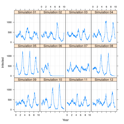
Note that the model contains no seasonality. Rather, the system experiences stochastic resonance, where the “noise” of stochastic state transitions stimulates a resonant frequency of the system (here, 2-3 years). For more information see here.

Sometimes epidemics die out. In fact, for this model, they will die out with probability = 1 as time goes to infinity!

library(lattice)

## lattice plot of results
plot(
    xyplot(I ~ time | sprintf("Simulation %02d",nsim),
        data=result.rep, type=c('l','g'), as.table=T,
        ylab='Infected', xlab='Year',
        scales=list(y=list(alternating=F))
    )
)

plot of chunk unnamed-chunk-4

tags: simulation basics

Extending R with C++ and Fortran — Dirk Eddelbuettel and JBrandon Duck-Mayr
Benchmarking Rcpp code with RcppClock — Zach DeBruine
Simulation Smoother using RcppArmadillo — Tomasz Woźniak